Introduction to Machine Learning Concepts | Learn Computer Academy

Earlier lessons described machine learning in general terms. This lesson goes into the actual categories machine learning falls into — conceptually, with no heavy mathematics required.

Supervised Learning

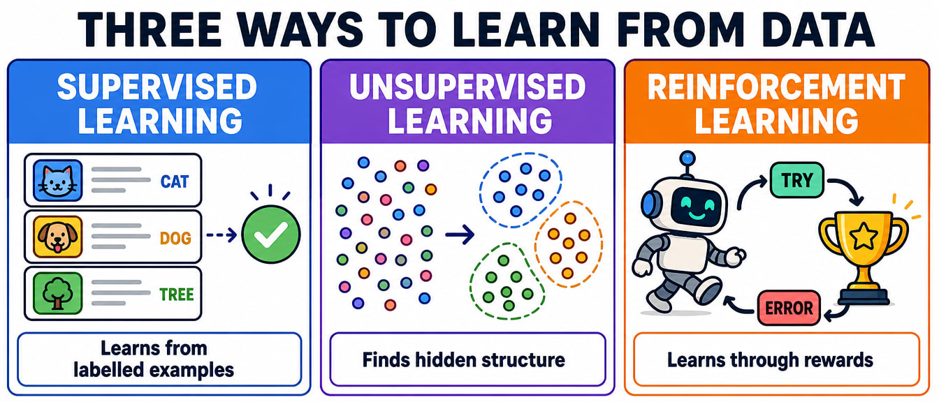
The model trains on labelled data — pairs of input and correct output — and learns to map one to the other. It splits into two kinds of problem:

Kind	What the output is	Examples
Classification	A category	Spam or not spam; cat or dog; disease present or not
Regression	A number	Predicting a house price; predicting delivery time; predicting an exam score from hours studied

A classic teaching example is the Titanic survival dataset — predicting who survived based on age, gender, and ticket class. It's a good example precisely because you already have intuitions to test ("women and children first" — does the data actually confirm that?).

Unsupervised Learning

No labels this time — the model finds hidden structure in data on its own.

Clustering — grouping similar items together. For example, grouping thousands of customers by purchase behaviour without knowing anything about who they are demographically.
Dimensionality reduction — compressing data with many measured features down to the few that actually capture most of the useful information.

Reinforcement Learning

An AI agent learns by trial and error — taking actions in an environment and receiving rewards or penalties based on the outcome. This is how systems learn to play games at a superhuman level, how some robots learn to walk, and how recommendation systems learn which content keeps someone engaged.

Infographic comparing three types of machine learning side by side — supervised learning trained on labelled input-output pairs, unsupervised learning finding hidden structure in unlabelled data, and reinforcement learning improving through trial-and-error rewards and penalties

Training, Testing, and the Overfitting Trap

Data is normally split into a training set (what the model actually learns from) and a separate test set it never sees during training — used afterward to check whether it actually learned general patterns rather than just memorising the training examples.

Two Ways Training Can Go Wrong

Overfitting is when a model performs great on training data but poorly on new data — it memorised specifics instead of learning the underlying pattern, like a student who memorises answers to last year's exam questions instead of understanding the subject. Underfitting is the opposite problem: the model is too simple to capture the pattern at all, performing poorly on both training and test data.

Neural Networks, Without the Maths

A neural network is organised into layers of simple mathematical units ("neurons"). Data enters at the first layer, passes through one or more "hidden" layers that combine it in increasingly abstract ways, and a final layer produces the output — a category, a number, or a probability for each possible answer. You don't need to understand the maths inside each neuron to have a working mental model: more layers and more neurons generally let a network learn more complex patterns, at the cost of needing more data and more computing power to train.

Watching a Real Classifier Train

This is genuinely one of the more satisfying things to see happen: a real neural network, trained live, for free, in a browser.

import tensorflow as tf
from tensorflow import keras

# Load 60,000 labelled images across 10 categories
(x_train, y_train), (x_test, y_test) = keras.datasets.cifar10.load_data()
x_train, x_test = x_train / 255.0, x_test / 255.0  # scale pixel values

model = keras.Sequential([
    keras.layers.Flatten(input_shape=(32, 32, 3)),
    keras.layers.Dense(128, activation='relu'),
    keras.layers.Dropout(0.2),          # helps reduce overfitting
    keras.layers.Dense(10, activation='softmax'),
])

model.compile(optimizer='adam',
              loss='sparse_categorical_crossentropy',
              metrics=['accuracy'])

history = model.fit(x_train, y_train, epochs=10, validation_split=0.1)

test_loss, test_acc = model.evaluate(x_test, y_test, verbose=0)
print(f"Test accuracy: {test_acc*100:.1f}%")

Watch the accuracy number as training runs: it typically starts around 35% after the first pass through the data and climbs toward 55% by the tenth. That may not sound impressive, but random guessing across 10 categories would only score about 10% — and this is a genuinely simple network with no advanced techniques applied.

You now understand the shape of machine learning as a field. The next lesson zooms in on the specific technology this whole section has been building toward: large language models and RAG, in real depth.